Defining the Question

Can we utilize computer vision to build a better prosthetic?

The Organization

For this project, I am working with RomboLabs on the University of Washington campus under Dr. Eric Rombokas. They are doing this research on behalf of the US Office of Veteran Affairs. Because the results of this research are still awaiting publication, I won’t be including any links to repos, though I will include a few code snippets for illustration.

Understanding the Problem

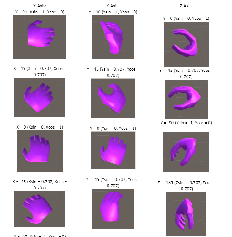
Prosthetics are an exciting field of study in the world of robotics. They show a marked and immediate impact on people’s lives, giving back vital pieces of humanity to those who have lost them. While they target a small portion of the population, the improvement that they offer is significant. However, they are far from flawless. There are many different approaches to this particular topic. For this project, we are looking at the more common hand replacement, which is a claw style prosthetic that is operated by a shrug mechanism. That is to say, the operator ‘shrugs’ to open and close the claw. These are fixed orientation, or if they change, typically it is done with the other hand manually rotating the wrist. We can already see some limitations.

Our Solution

Our hope is to utilize computer vision and simple robotics to generate a wrist mechanism that will evaluate objects and then predict the proper rotation needed to interact with the given object. There are several individuals working on this team, and I won’t go into details on the robotics engineering specifically here. For our portion, we have a virtual reality headset and large glove utilizing a Unity program. A test subject gets into the rig and is show a variety of objects with different orientations. We then track their retina and their hand position. There are a few difficulties with tracking eye data, and we should discuss them briefly now. The human eye actually sees a very small portion of our field of vision at any given time. What we think we see is largely an extrapolation our brain generates based on changes to sees from one moment to the next. The reason for this is a movement the eye does called saccades; that is the eye jumps around to better build the image of thing you are seeing. These motions are involuntary and we are more or less unaware of them. These motions are one of the reason why humans track movement better than stationary objects, and why we have a specific frames-per-second that we can observe. Because of the saccades, we can’t simply take a snapshot of where the eye was to see what you were actually looking at since there is a high probability that your eye was performing one of these saccades. Therefore, we take a second worth of data at the moment of a positive grip and record that. The hand data is very similar throughout this second, but we have 60 frames of visual data to layer over it. We then take the number of times that the eye fell on a specific point and the length of time it stayed there and plot it against the object.

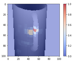
While we are tracking the eye movements, we are also tracking the hand and forearm movements. The glove is outfitted with over 70 sensors to track each joint, rotation, and orientation on each of the elements of the hand. Due to how Unity and the glove interact, each of these joints data is broken into two elements for Sin and Cos to better express these points. Some of this data is sparse or not terribly relevant. Hand kinesthetics are unique; for grip types, often times the thumb and first finger matter a great deal, but often the rest of the fingers are slaved to the first two fingers. There are also specific rotations of individual joints that aren’t relevant.

Using the hand kinesthetics as our labels, we are trying to use the eye data as our predictive data. Essentially, we are going to take visual data from sensors moving forward to predict what the hand should be doing. We are going to try a regression neural network to predict the range of each of these joints. Our other approach is going to be a categorical approach, where we take the hand data and push it through specific algorithms to generate three discrete categories: Vertical, Horizontal, and Slanted.

My focus for this project is the control aspects of the categorical neural network.

The Software Engineering

I tried a bunch of different approaches for the hand data. As a preprocessing method, we attempted to apply a clustering to see if we could find patterns in the data. Because the hand data covers 156 different aspects, traditional clustering methods didn’t yield much positive results. However, we did attempt to utilize the UMAP library to build a better manifold type clustering for the high dimensionality of the data. UMAP is a bit contraversal in its effectiveness, but we at least got interesting results on some of our test data. We executed this using the following code (‘result’ is the dataframe of our shaped hand observations) :

from sklearn.decomposition import PCA
import numpy as np
import matplotlib.pyplot as plt
import seaborn as sns
%matplotlib inline

# Dimension reduction and clustering libraries
import umap
import hdbscan
import sklearn.cluster as cluster
from sklearn.metrics import adjusted_rand_score, adjusted_mutual_info_score

standard_embedding = umap.UMAP(random_state=42).fit_transform(result)
plt.scatter(standard_embedding[:, 0], standard_embedding[:, 1], s=0.1, cmap='Spectral');

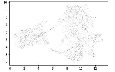
I apologize for the small nature of these images; the take-away here is that UMAP was far more effective at plotting these points than traditional methods. To break them into clusters, we applied the following code:

clusterable_embedding = umap.UMAP(
    n_neighbors=30,
    min_dist=0.0,
    n_components=2,
    random_state=42,
).fit_transform(result)

labels = hdbscan.HDBSCAN(
    min_samples=10,
    min_cluster_size=500,
).fit_predict(clusterable_embedding)

clustered = (labels >= 0)
plt.scatter(standard_embedding[~clustered, 0],
            standard_embedding[~clustered, 1],
            c=(0.5, 0.5, 0.5),
            s=0.1,
            alpha=0.5)
plt.scatter(standard_embedding[clustered, 0],
            standard_embedding[clustered, 1],
            c=labels[clustered],
            s=0.1,
            cmap='Spectral');

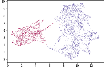
These cluster didn’t determine our labels purely on their own, but these results did help educate our process.

With our labels generated for the vision data, we then looked to build our neural network. Because the heat/depth of the visual data yields a 2x101x101 matrix, we elected to use a convolutional neutral network. Because of the various aspects that we could use, I settled on attempting a grid-search method to trim down the hyper parameters. TensorFlow and Keras work well with scikit-learn, provided you import a specific wrapper. Grid Search is a method of model selection wherein you dictate a number of parameters and ranges for those parameters, and you computer will build the models and test them. The results are then fed back to you in a very readable way. This is a good method to rapid try a variety of approaches without generating a massive amount of models. Typically, these are done in waves, where you test specific parameters in batches and use the best results to educate the next set of hyperparameters you want to test. For the purposes of this post, we will be covering the first set of hyperparameters that we checked. Future postings will cover the second set of hyperparameters and the final model architecture that we settled on.

To begin, we have a variety of models that we need to pull in:

import numpy as np
import pandas as pd
from sklearn.model_selection import GridSearchCV, train_test_split
from tensorflow.keras.models import Sequential
from tensorflow.keras.layers import Activation, Dense, Flatten, Conv2D, MaxPooling2D, Dropout
from tensorflow.keras.optimizers import SGD, Adam, Adamax, Adagrad, Ftrl
from tensorflow.keras.initializers import RandomNormal, RandomUniform, TruncatedNormal
from tensorflow.keras.wrappers.scikit_learn import KerasClassifier
import tensorflow as tf
from tensorboard.plugins.hparams import api as hp

Certain other libraries were used to shape the data correctly and bring it into the script (like os or datetime), but have been omitted for brevity.

With our base libraries in place, we then bring in the data and labels, ensure that they line up properly and are shaped properly. Then we decide what our first batch will be testing. The most common hyperparameters to test are the number of nodes in each layer, the number of layers in the model, and the number of epochs to train. For the purposes of the first batch, we will be testing the following:

• num_units= the number of nodes per layer
• learning_rate= the learning rate for the optimizer
• opt= a range of optimizing functions
• layers= Additional layers past the flattening layer. Our base model will have 1 by default.
• initializer= different weight initializing functions.

These are defined in the following way:

HP_NUM_UNITS = hp.HParam('num_units', hp.Discrete([16,32,64,512]))
HP_LEARNING_RATE = hp.HParam('learning_rate', hp.RealInterval(0.001, 0.01))
HP_OPTIMIZER = hp.HParam('optimizer', hp.Discrete(['adam', 'adamax', 'sgd', 'adagrad', 'ftrl']))
HP_LAYERS = hp.HParam('layers', hp.Discrete([0,1,2,4,5]))
HP_INITIALIZER = hp.HParam('initializer', hp.Discrete(['truncatednormal', 'randomnormal', 'randomuniform']))
METRIC_ACCURACY = 'accuracy'

with tf.summary.create_file_writer('logs/hparam_tuning').as_default():
  hp.hparams_config(
      hparams=[HP_NUM_UNITS, HP_LEARNING_RATE, HP_OPTIMIZER, HP_LAYERS, HP_INITIALIZER],
      metrics=[hp.Metric(METRIC_ACCURACY, display_name='Accuracy')]
  )

We then need to build a function that will build each of the models to be tested. Certain elements of the model will be constant, but we will be testing different elements of them in future models. Specifically, the convolutional portion of the network is constant. A traditional convolutional network has a Conv layers paired with MaxPooling layers before eventually being flattened and then fed through a traditional neutral network Dense layer model. We will be using the Sequential model from Keras for ease of use.

def create_model(hparams):
  init_name = hparams[HP_INITIALIZER]
  
  model = tf.keras.Sequential([
                               tf.keras.layers.Conv2D(hparams[HP_NUM_UNITS], kernel_size=(3,3),
                                                      kernel_initializer=init_name,
                                                      activation='relu', 
                                                      data_format='channels_first', 
                                                      input_shape=X_train[0].shape),
                               tf.keras.layers.MaxPooling2D(pool_size=(2,2), data_format='channels_first'),
                               tf.keras.layers.Dropout(0.1),
                               tf.keras.layers.Conv2D(32, kernel_size=(3,3), data_format='channels_first', activation='relu'),
                               tf.keras.layers.MaxPooling2D(pool_size=(2,2), data_format='channels_first'),
                               tf.keras.layers.Conv2D(32, kernel_size=(3,3), data_format='channels_first', activation='relu'),
                               tf.keras.layers.Flatten(),
                               tf.keras.layers.Dense(hparams[HP_NUM_UNITS], activation='relu'),
                               tf.keras.layers.Dropout(0.1),
  ])

  for layer in range(hparams[HP_LAYERS]):
    model.add(Dense(hparams[HP_NUM_UNITS], activation='relu')),
    model.add(Dropout(0.1))

  model.add(Dense(3, activation='softmax'))

  opt_name = hparams[HP_OPTIMIZER]
  lr = hparams[HP_LEARNING_RATE]

  if opt_name == 'adam':
    opt = tf.keras.optimizers.Adam(learning_rate=lr)
  elif opt_name == 'adamax':
    opt = tf.keras.optimizers.Adamax(learning_rate=lr)
  elif opt_name == 'adagrad':
    opt = tf.keras.optimizers.Adagrad(learning_rate=lr)
  elif opt_name == 'ftrl':
    opt = tf.keras.optimizers.Ftrl(learning_rate=lr)
  elif opt_name == 'sgd':
    opt = tf.keras.optimizers.SGD(learning_rate=lr)
  else:
    raise ValueError(f'Unexpected optimizer name: {opt_name}')

  model.compile(
      optimizer= opt,
      loss= 'sparse_categorical_crossentropy',
      metrics = ['accuracy']
  )

  model.fit(X_train, y_train, epochs=10)

  _, accuracy = model.evaluate(X_test, y_test)

  return accuracy

Note that our loss function is sparse_categorical_crossentropy due to the nature of our labels. I have also implemented numerous dropout layers. This is in an attempt to avoid overfitting as our data at the moment is not very deep. I have also set an arbitrary number of epochs at 10; when the final model is built we will implement early stopping, so this exists purely for the grid search. Further, the only activation function we are testing is ReLU and softmax. Softmax is because of the number of categories our labels have, and ReLU has pretty consistently out performed other functions. For the next set of batches, I may test different activations, but for now I am comfortable with ReLU. Also, because these models aren’t being stored in any way, all we care about is the accuracy of the given models, so that is all we are returning. Our data is then split, confirmed that the shapes are consistent and then we create the helper function that will allow TensorBoard to operate properly.

def run(run_dir, hparams):
  with tf.summary.create_file_writer(run_dir).as_default():
    hp.hparams(hparams)
    accuracy = create_model(hparams)
    tf.summary.scalar(METRIC_ACCURACY, accuracy, step=1)

And now we’re ready to begin our search. Ensure you load tensorboard before you start this process, as I have had issues if I have tried it after the logs were generated in the past.

%load_ext tensorboard

A series of nested for loops are necessary for each element to be tested, which ensures that this process can be computationally expensive and long. It is strongly recommended that you utilize your GPU to speed this up.

session_num = 0
for num_units in HP_NUM_UNITS.domain.values:
  for learning_rate in (HP_LEARNING_RATE.domain.min_value, HP_LEARNING_RATE.domain.max_value):
    for optimizer in HP_OPTIMIZER.domain.values:
      for layers in HP_LAYERS.domain.values:
        for initalizers in HP_INITIALIZER.domain.values:
          hparams = {
              HP_NUM_UNITS: num_units,
              HP_LEARNING_RATE: learning_rate,
              HP_OPTIMIZER: optimizer,
              HP_LAYERS: layers,
              HP_INITIALIZER: initalizers,
          }
          run_name = f"run-{session_num}"
          print(f'--- Starting Trial: {run_name}')
          print({h.name: hparams[h] for h in hparams})
          run('logs/hparam_tuning/' + run_name, hparams)
          session_num += 1

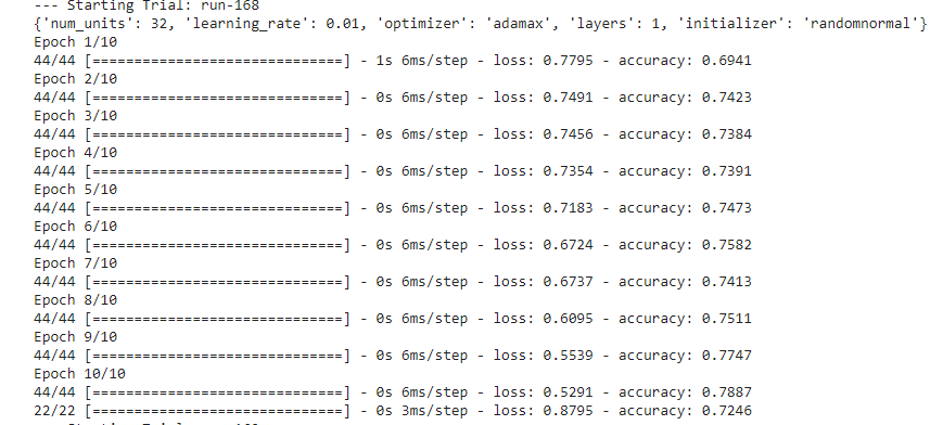
If done properly, your machine should start executing hundreds of trials that look like the following:

There is a bunch of good data to be had in these. Once all of the trials are completed, activate your tensorboard to review your results:

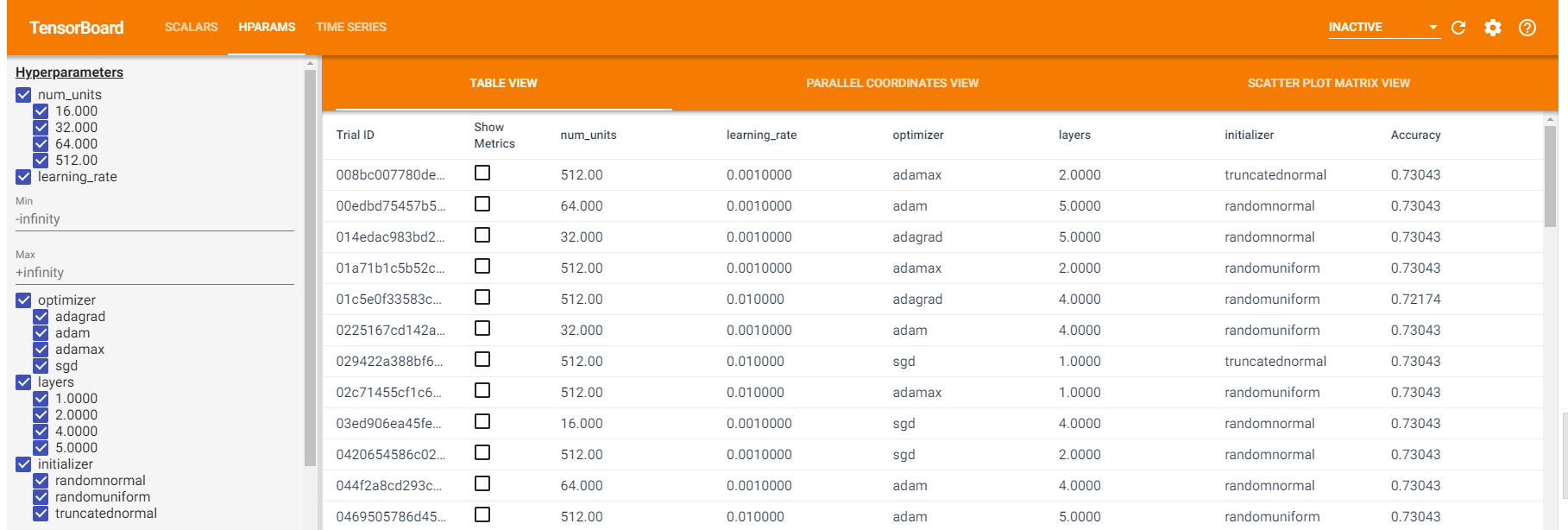
Our best results for this trials came with the following (some of which are not at all surprising) model architectures:

• High nodes
• Low layers
• Adam or AdaMax
• RandomUniform or Truncated
• And learning rates around .001

The Next Steps

Using the above guidelines, we will begin a second batch of tests to see which models perform the best. It is my intention to test the depth of the convolutional aspects of the model primarily to see if we can squeeze out better performance if we shorten the convolutions or remove the dropout layers. As previously stated, we will implement early stopping for our actual model, so epochs aren’t a hyperparameter that we will worry overly much about.

This project is not completed and still awaiting publication. The next steps and final model will be discussed in future blog posts on this board.